Optional Lab: Model Representation

Goals

In this lab you will:

• Learn to implement the model $f_{w,b}$ for linear regression with one variable

Notation

Here is a summary of some of the notation you will encounter.

|General
Notation | Description| Python (if applicable) | |: ------------|: ------------------------------------------------------------|| | $a$ | scalar, non bold || | $\mathbf{a}$ | vector, bold || | Regression | | | | | $\mathbf{x}$ | Training Example feature values (in this lab - Size (1000 sqft)) | x_train |
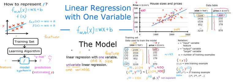
| $\mathbf{y}$ | Training Example targets (in this lab Price (1000s of dollars)). | y_train | $x^{(i)}$, $y^{(i)}$ | $i_{th}$Training Example | x_i, y_i| | m | Number of training examples | m| | $w$ | parameter: weight, | w | | $b$ | parameter: bias | b |
| $f_{w,b}(x^{(i)})$ | The result of the model evaluation at $x^{(i)}$ parameterized by $w,b$: $f_{w,b}(x^{(i)}) = wx^{(i)}+b$ | f_wb |

Tools

In this lab you will make use of:

• NumPy, a popular library for scientific computing
• Matplotlib, a popular library for plotting data

import numpy as np
import matplotlib.pyplot as plt
plt.style.use('./deeplearning.mplstyle')

Problem Statement

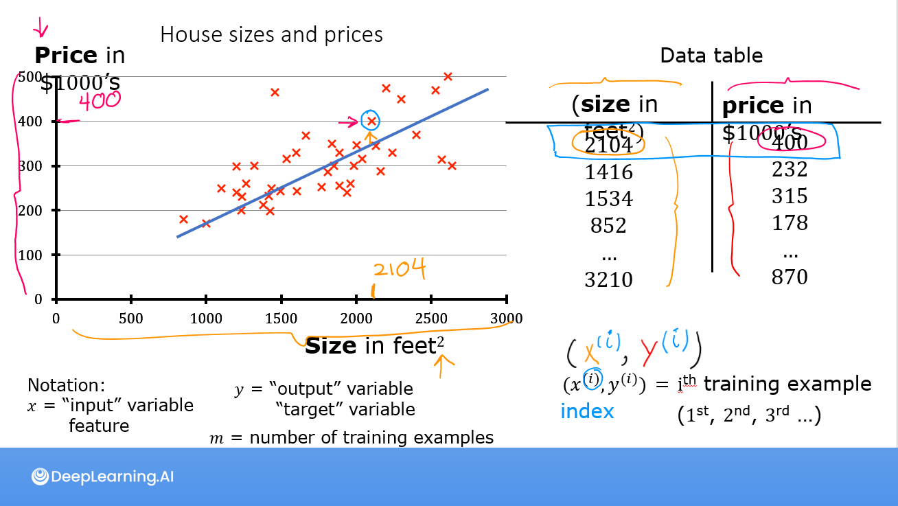
As in the lecture, you will use the motivating example of housing price prediction.
This lab will use a simple data set with only two data points - a house with 1000 square feet(sqft) sold for \$300,000 and a house with 2000 square feet sold for \$500,000. These two points will constitute our data or training set. In this lab, the units of size are 1000 sqft and the units of price are 1000s of dollars.

Size (1000 sqft)	Price (1000s of dollars)
1.0	300
2.0	500

You would like to fit a linear regression model (shown above as the blue straight line) through these two points, so you can then predict price for other houses - say, a house with 1200 sqft.

Please run the following code cell to create your x_train and y_train variables. The data is stored in one-dimensional NumPy arrays.

# x_train is the input variable (size in 1000 square feet)
# y_train is the target (price in 1000s of dollars)
x_train = np.array([1.0, 2.0])
y_train = np.array([300.0, 500.0])
print(f"x_train = {x_train}")
print(f"y_train = {y_train}")

Note: The course will frequently utilize the python 'f-string' output formatting described here when printing. The content between the curly braces is evaluated when producing the output.

Number of training examples m

You will use m to denote the number of training examples. Numpy arrays have a .shape parameter. x_train.shape returns a python tuple with an entry for each dimension. x_train.shape[0] is the length of the array and number of examples as shown below.

# m is the number of training examples
print(f"x_train.shape: {x_train.shape}")
m = x_train.shape[0]
print(f"Number of training examples is: {m}")

One can also use the Python len() function as shown below.

# m is the number of training examples
m = len(x_train)
print(f"Number of training examples is: {m}")

Training example x_i, y_i

You will use (x$^{(i)}$, y$^{(i)}$) to denote the $i^{th}$ training example. Since Python is zero indexed, (x$^{(0)}$, y$^{(0)}$) is (1.0, 300.0) and (x$^{(1)}$, y$^{(1)}$) is (2.0, 500.0).

To access a value in a Numpy array, one indexes the array with the desired offset. For example the syntax to access location zero of x_train is x_train[0]. Run the next code block below to get the $i^{th}$ training example.

i = 0 # Change this to 1 to see (x^1, y^1)

x_i = x_train[i]
y_i = y_train[i]
print(f"(x^({i}), y^({i})) = ({x_i}, {y_i})")

Plotting the data

You can plot these two points using the scatter() function in the matplotlib library, as shown in the cell below.

• The function arguments marker and c show the points as red crosses (the default is blue dots).

You can use other functions in the matplotlib library to set the title and labels to display

# Plot the data points
plt.scatter(x_train, y_train, marker='x', c='r')
# Set the title
plt.title("Housing Prices")
# Set the y-axis label
plt.ylabel('Price (in 1000s of dollars)')
# Set the x-axis label
plt.xlabel('Size (1000 sqft)')
plt.show()

Model function

As described in lecture, the model function for linear regression (which is a function that maps from x to y) is represented as

$$ f_{w,b}(x^{(i)}) = wx^{(i)} + b \tag{1}$$

The formula above is how you can represent straight lines - different values of $w$ and $b$ give you different straight lines on the plot.

Let's try to get a better intuition for this through the code blocks below. Let's start with $w = 100$ and $b = 100$.

Note: You can come back to this cell to adjust the model's w and b parameters

w = 100
b = 100
print(f"w: {w}")
print(f"b: {b}")

Now, let's compute the value of $f_{w,b}(x^{(i)})$ for your two data points. You can explicitly write this out for each data point as -

for $x^{(0)}$, f_wb = w * x[0] + b

for $x^{(1)}$, f_wb = w * x[1] + b

For a large number of data points, this can get unwieldy and repetitive. So instead, you can calculate the function output in a for loop as shown in the compute_model_output function below.

Note: The argument description (ndarray (m,)) describes a Numpy n-dimensional array of shape (m,). (scalar) describes an argument without dimensions, just a magnitude.
Note: np.zero(n) will return a one-dimensional numpy array with $n$ entries

def compute_model_output(x, w, b):
    """
    Computes the prediction of a linear model
    Args:
      x (ndarray (m,)): Data, m examples 
      w,b (scalar)    : model parameters  
    Returns
      y (ndarray (m,)): target values
    """
    m = x.shape[0]
    f_wb = np.zeros(m)
    for i in range(m):
        f_wb[i] = w * x[i] + b
        
    return f_wb

Now let's call the compute_model_output function and plot the output..

tmp_f_wb = compute_model_output(x_train, w, b,)

# Plot our model prediction
plt.plot(x_train, tmp_f_wb, c='b',label='Our Prediction')

# Plot the data points
plt.scatter(x_train, y_train, marker='x', c='r',label='Actual Values')

# Set the title
plt.title("Housing Prices")
# Set the y-axis label
plt.ylabel('Price (in 1000s of dollars)')
# Set the x-axis label
plt.xlabel('Size (1000 sqft)')
plt.legend()
plt.show()

As you can see, setting $w = 100$ and $b = 100$ does not result in a line that fits our data.

Challenge

Try experimenting with different values of $w$ and $b$. What should the values be for a line that fits our data?

Tip:

You can use your mouse to click on the triangle to the left of the green "Hints" below to reveal some hints for choosing b and w.

Hints

• Try $w = 200$ and $b = 100$

Prediction

Now that we have a model, we can use it to make our original prediction. Let's predict the price of a house with 1200 sqft. Since the units of $x$ are in 1000's of sqft, $x$ is 1.2.

w = 200                         
b = 100    
x_i = 1.2
cost_1200sqft = w * x_i + b    

print(f"${cost_1200sqft:.0f} thousand dollars")

Congratulations!

In this lab you have learned:

• Linear regression builds a model which establishes a relationship between features and targets
  • In the example above, the feature was house size and the target was house price
  • for simple linear regression, the model has two parameters $w$ and $b$ whose values are 'fit' using training data.
  • once a model's parameters have been determined, the model can be used to make predictions on novel data.